Chapter 9 Water Quality Modelling

9.1. Introduction

Natural systems are very complicated and high-organized systems. Water quality models try to simulate changes in the pollutants concentration as they move through the environment. A pollutant entering the environment may increase or decrease its concentration due to a large variety of mechanisms. The fate of pollutants is the resultant of interactions between mass transfer and kinetic processes. All these changes are the subject of water quality modelling.

Modelling is a continuous process of developing models in times parallel with the increase of the available information and knowledge about the simulation system, which more and more adequate to describe the real process. The focus here is the user to receive the basic knowledge about water quality modelling by means of introducting the purpose, type, structure and application of the water quality models.

9.2 Why Model ?

Mathematical models are a means for governmental institutions to gain the best social and economic solutions of water problems and play very important role for the integrated watershed management. A model is a system of equations, relationships and observed monitoring data, created for description of the natural system, for demonstration and checking of its behaviour under different conditions in time and in suitable type with significant economy of money and time.

The use of mathematical models is the shortest way to:

simulate the effects of different scenarios on water quality for a river basin;
choose solutions where and how to invest for water quality improvement on the basis of comparison among needs for water with given quality and investment option;
assess the value of parameters, for which there is limited information.

9.3. Purpose of water quality modelling

The purpose of modelling should be clear and well defined to achieve maximum simplicity consistent with the required degree of accuracy and detail in the process of description of the natural system. In general, the purpose of modelling falls into one of the following categories (Zheng & Bennett, 1995):

In a scientific sense - to develop a clear conceptual model based on all available information as well as to understand more fully the transport regime of the pollutant: to test hypotheses, to ensure that they are consistent with governing principals and observations, and to quantify the dominant controlling processes. Without this understanding, a simulation code can be used only as a black-box, and this clearly limits intelligent application of the model;
Often in connection with efforts to assign responsibility or assess exposures, to reconstruct the history of pollutant transport, to establish time ranges within which an event could have begun, or within which contaminants could have reached specified level in certain areas;
Future contaminant distributions must be calculated, either under existing conditions or with engineering intervention to control the source or alter the flow regime. These include for example the choice of used computer code, the way of discretization, the level of effort required in model calibration, and the analysis of the appropriated assumptions. By definition a model is a simplified approximation to the real system. A simple model is always preferred to complex model, as long as it captures the essence of the problem. An overly complex model not only increases computational time and costs, but also introduces additional uncertainties if detailed data are not available.

9.4. Modelling fundamentals

The fundamental principles for water quantity and quality modelling are:

conservation of energy states (first law of thermodynamic);
conservation of mass states (mass balance models) and
conservation of momentum states (Newton's first law of motion).

9.5. Creation of water quality models

The key elements for creation of the suitable water quality models are related with the good knowledge about a change in state of a system, presented with the difference in properties between the final and the beginning state. The process of model building is an iterative process, which starts with expression of a working hypothesis, typically based on a priori knowledge about the system in the form of mathematical model. An experiment is like a window through which the nature is viewed. Our view is never perfect. Interaction between experimental data collection and data analysis provides the opportunity for improving precision by shifting emphasis to different variables, making repeated observations, and adjusting experimental conditions. The assessment of water quality is always related with the determination of water flow characteristics. It is not possible to assess water quality without evaluation of the water quantity. That is why the water quality modelling includes as a main part the water quantity modelling, which gives the answer how water movement affects the concentration of the dissolved and suspended constrains.

The creation of a water quality model involves the following two stages:

Analysis of the system - this may be theoretical, observational, or experimental;
Synthesis of a mathematical replica of the system.

The main steps of model building may be explained as follows (James, 1996):

Formulation of objectives - As more precisely the objectives are formulated, preferably in quantitative terms, the more satisfactory model is possible to be created and adapted;
Review of theoretical background - It should include an analysis of the processes affecting water quality, method of representation, and appropriate ranges for any model parameter, review and compile all relevant information at both local and regional scales;
Formulation of the model - This step involves a decision about the type of model, elimination of the relationships that do not affect the output results, examination of alternative types of models and careful relationships of base data collection. This information is integrated into a conceptual model, in general through the introduction of simplifying assumptions and qualitative interpretations regarding the flow and the transport process.
Creation of a model structure - Generally the process begins by identifying the large subdivisions of a model and proceeds by fitting these together in diagrammatic form with a flow chart. It is better the model to be created from different modules (separated parts) and every part to be developed, tested and calibrated apart.
Formulation of equations - On the basis of the review of theory and the model structure it is possible to state the relationships involved in some formal mathematical or statistical way. Adoption of a hierarchical approach to this process often results in a clearer set of equations in which the influence of primary and secondary relations can be more easily appreciated. Some preliminary data may be needed to guide the choice.
Formulation of methods of solution - Only in a few special cases it may be possible to solve the equations analytically, but most models involve the use of numerical methods for solving partial differential equations, interpolation, etc. The choice of the appropriate numerical technique is crucial for numerical stability and accuracy and also for minimizing computational effort.
Selection of a computer code - The decision depends on the project goals. If a modelling is intended only to provide a first approximation, a simple code may be appropriate. The form of input and output results, and the choice of the language, are in dependence of the available facilities. The simplest programming language is BASIC, which together with QBASIC is a power tool for many modelling purposes.
Calibration of the model - It is essential that completely independent data sets are used for the calibration procedure. Calibration is one of the most critical, difficult, and valuable steps in the model application process. After a pollutant transport model is calibrated to a satisfactory degree, it is often applied to predict and simulate the future contaminant migration.
Validation of the model - It is impossible to apply the model as representative without suitable proof. The validation of the model depends on the local possibilities. Model validation, evaluation, confirmation, or testing is the process of assessing the degree of reliability of the calibrated model using one or more independent data sets. Ideally it is possible to compare the output results from the model with the observed data.
Statistical assessment of paired observations and simulations - The basic statistical parameters and goodness-of-fit criteria are: average error, standard deviation, correlation coefficient, index of agreement, per cent deviation per year by flow and pollutants, and others.
Sensitivity analysis -This procedure is used before and after calibration mainly to test the responsiveness and sensitivity of the numerical model to every input parameter. The sensitivity analysis is useful for: examining the likely uncertainty in simulation results due to uncertainty in model input parameters, and examining how well parameters are likely to be estimated from the available data for model calibration. Sensitivity analysis provides important information on how uncertainties in the model parameters affect the model results. If the model results are highly sensitive to a particular parameter, the uncertainty associated with that parameter will significantly affect the ability of the model to make meaningful interpretations and predictions. Sensitivity analysis is the mean of determining the model parameters.

9.6. Basic equations for water quality modelling

The instantaneous equations for fluid flow and pollutant transport are:

Conservation equations, which describe the conservation of momentum, water mass, heat energy, and constituent mass;
Equation of continuity of water.

9.7. Techniques of solving of the basic equations

The used solution techniques for solving the basic equations are:

Analytical solution - up to now is obtained after simplification of the differential governing equations to a level at which an analytical solution is possible;
Numerical solution - depends of the type of the system equations. In case of creating the system of differential equations they are converted into algebraic difference forms using one of the most common finite-difference approximations - Runge-Kuta method and others.

The simplifications are related to the resolution of water quality processes in time and space, and the numerical techniques used to solve the governing equations.

9.8. Types and sources of uncertainty in modelling

All simulations are subject to uncertainty. Hydraulic and transport parameters and boundary conditions are never known in sufficient detail and the existing distributions of the pollutants are often poorly understood.

Uncertainty in the results may be classified into two general categories:

Those associated with model input parameters and
Those associated with numerical and conceptual difficulties in modelling pollutant transport.

9.9. Types of water quality modelling

The field of the water quality models is very large and includes different kind of models in dependence of the level of the input and output information, the complexity of the modelled events, the modelled water body, the used mathematical methods, the type of the basic equations, the aim of the modelling, the structure of the modelling system, the scale of interest in steady-state or non-steady state conditions and others. Many different types of water quality models are available so it is not possible to give a simple classification (Figure 9.1).

The optimization models are a group of mathematical techniques used to obtain the least costly solution to some allocation situation. The simulation models describe all models representing water quality changes in some mathematical form including all types of mechanistic models in which the processes are deterministically represented, and also statistical models.

9.9.1. General classification of water quality models by types

9.9.1.1. Mechanistic models

Mechanistic water quality models are models that by means of mathematical tools express the mechanisms of the process that cause changes on water quality and lead to establish the relationship "cause-and-effect". The mechanistic models have some advantages:

To gain insights and increased understanding of the water quality of a particular stream;
To provide information on "cause-and-effect" relationships;
To indicate what is not understood;
To provide a predictive capability.

Figure 9.1 Classifications of Water Quality Models

9.9.1.2. Empirical models

Empirical models are "black-box" models. Purely empirical models, such as many statistical models, allow description of the fixed relationships between input data and output results with a minimum of understanding about how the system works. Statistical models estimate the parameters through statistical analysis and then check the adequacy of the model. One of the principal restrictions of the empirical models is that they cannot be implemented to other close systems or for data out of the range used for creation of the model (J. Martin, 1999).

The common tendency is the model to be more fundamental and less empirical. From the practical point of view the water quality management models will have empirical character in future.

9.1.1.3. Deterministic models

Deterministic models have a fixed relationship between input data and output results, which may be empirical or mechanistic.

9.1.1.4. Stochastic models

Stochastic models contain some random elements. They are divided into: steady-state Monte-Carlo simulation models, using a mass balance model, which generate an output result with varying input conditions in the form of a frequency distribution of the pollutant concentration, and dynamic time series simulation models, using a dynamic finite difference model.

9.9.2. Types of water quality models in dependence of the simulated waterbody

9.9.2.1. Models of water quality in rivers

Modelling framework of water quality in rivers includes two basic steps:

Simulation of the flow regime to create clear picture of water movement together with calibration and validation of the model (including hydrologic simulation of runoff, groundwater and stream flow; hydraulic simulation of water surface; average velocities; average depths and etc. for every reach of the river).
Simulation of the water quality in every reach of the river together with calibration and validation of the model. This procedure includes simulation of the most important types of pollutants, loads entering and leaving parallel with reactions and transformations, plus mass exchange between water and atmosphere, and water and benthos, and takes into account the self-purification capability of the flow.

9.9.2.2. Models of water quality in estuaries

Estuaries are a distinct part of the river system: the transition zone between rivers and saline habitats. Water quality models include:

Simulation of the estuarine hydraulics for every type of estuary (water levels and water depths, velocities and directions) and
Simulation of estuarine water quality models. They are: black-box models, box or segment models, moving segments models and finite difference or finite element models on the basis of salinities, temperature, water quality parameters like DO, BOD, loads of pollutants entering the estuary, freshwater flows from any significant tributary, estimation of coefficients of dispersion, re-aeration, etc.

9.9.2.3. Models of water quality in reservoirs and lakes

Physical models - modelling of overall temperature, thermal structure models, hydrodynamic models;
Chemical models - simulating the concentration of various substances, mainly nutrients and toxins for the prediction of eutrophication;
Biological models - algal growth model, respiration, sedimentation, nutrient recycle, oxygen balance model;
Lake models - long-term planning models (used to forecast the increase in algal growth to predict the effect of some management decision), short-term operational models (used for day-to-day control of algal growth in an already eutrophic reservoir) and tropical lakes and reservoirs models.

9.9.2.4. Models of water quality in groundwater

Simulation of groundwater flow motion - steady-state flow model for determination of average groundwater fluxes and average water velocity;
Simulation of contaminant transport - transport by advection, transport by dispersion, production and decay of the transported species, adsorption, the dual porosity model.

9.9.2.5. Models of water quality in runoff

Simulation of runoff - a surface runoff model;
Simulation of the runoff quality model - an erosion and sediment delivery model and a nutrient production model.

9.9.3. Types of water quality models by function of pollutants

Mainly by function of pollutants the water quality models are divided into two broad groups:

Water quality models for estimation non-point source pollution of stream flow;
Water quality models for estimation point source pollution.

Usually these two models work together, included in one common decision making system. It evaluates the water quality in every reach of the river, resultant from point and non-point sources of pollution together with integration of the self-purification capability of the stream flow and all the physical, chemical and biological processes simulations.

9.10. Aquatic data requirements

Monitoring of aquatic environments generally produces data in the form of repeated observations of some parameters at various sampling points. The data are divided into three types:

Continuous records - These data need to be discretized into average values over time intervals so that they can be analysed. Care is needed in the choice of time interval;
Discrete records from samples taken at particular moments;
Cumulative records like daily rainfall where the parameter is already discretized and averaged by the sampling procedure.

The analysis of the monitoring data has to be made. First the data are plotted on a time basis (Figure 9.2). Visual inspection is an essential preliminary step to the more detailed analysis related with the assessment of the common trend of changing and the notation of the measurements, declined from the trend.

Figure 9.2 Analysis of observed data

9.11. Simulation of water quality in rivers

For better understanding some examples are presented below with some characteristics of a special water quality assessment system REKA (River Environmental Knowledge and Assessment), developed for the Yantra river basin in Bulgaria to evaluate non-point and point sources of pollution in a media of Geographical Information Systems (GIS). REKA has two sub-components: BISTRA (Basin Impacts of Simulated Transport from Rural Areas) and VODA (Validation and Optimization for Decision Analysis). The system goal was to create an approach to assess the water quality in various river reaches in dependence of future climate variability and socio-economic changes.

9.11.1. Data Base for the REKA System

Application of the REKA model requires the availability of a comprehensive, well-structured database for assessment of the water quality of a given watershed and river reach. All these spatial data are presented as ArcView map layers giving the geographical position of the objects. The numerical data related with these objects are structured in attribute tables attached to the layers. Some required input layers are presented for Yantra river basin, in Bulgaria.

9.11.1.1. Territory

The total Yantra watershed as well as the tributary subbasins, the latter arranged for running the non-point source pollution model, are represented in Figure 9.3.

Figure 9.3 subbasins and river set

9.11.1.2. Digital Elevation Model

The Digital Elevation Model (DEM) supplies very important information about the slopes of the terrain and the river reaches (Figure 9.4).

Figure 9.4 DEM model

9.11.1.3. Hydrological and Meteorological Data

Flow monitoring data are needed for calibration of the stream flow results. They are related to the gauge stations, defined geographically as a separate gauge station layer. The daily rainfall and temperature data are presented for every meteorological station.

9. 11.1.4. Land Use

The land use data were supplied from digitized land use maps entered in GIS layers. Typically, land use maps are created by specialized services using topographic base maps and field studies. When available, satellite images are useful for improving land use maps (Figure 9.5).

Figure 9.5 Land use map

9.11.1.5. Soil Data

BISTRA requires a large number of soil characteristics specified by soil types. Figure 9.6 represents the Yantra River basin soil map.

Figure 9.6 Soil map

9.11.1.6. Demographic Data and Administrative Divisions

The demographic data include settlements and the administrative division of the watershed. The settlements are organized in 26 municipalities and in 6 counties and classified by analysis of the Land satellite imagery in 3 types:

low density,
medium density and
high density.

9.11.1.7 Water Quality Data

They are gathered for every water quality monitoring points for calibration and validation of the BISTRA and VODA models.

9.11.2 BISTRA - Water quality model for estimation of non-point source pollution of stream flow

BISTRA was developed for estimation of the non-point pollution in the Yantra River Basin on the basis of the GWLF model/GISArcView Interface. BISTRA assesses stream flow, nutrients and sediments in the 75 regions of the basin (Figure 9.7), for every outlet of the subbasins. The input information includes 10 layers and related attribute tables and some specific parameters, for which values were evaluated during the calibration procedure.

Figure 9.7 subbasins watersheds

9.11.2.1. Possibilities of the model

The BISTRA model allows:

one or a group of basins to be assessed;
automatic creation of the input files;
selection of the time length of simulation, duration of the growing season and management practices within subbasins;
designating agricultural lands with or without manure and selection of the time of manure;
choosing the type of simulation;
creation of output information;
visualization of the nutrient pollution variability along the whole river network and provision of output files - the input file for VODA model.

9.11.2.2. Application of the model

The application of the BISTRA model to the Yantra River basin includes:

automatic identification of the appropriate input data;
calibration and validation of the BISTRA model.

9.11.2.3. Choice of subbasins for the BISTRA calibration

Choice of subbasins was based on the following important requirements:

The outlet of the subbasin should coincide with a gauge station for the purpose of comparing the simulated and observed flows;
The runoff of the watershed should not be regulated by anthropogenic activities;
The subbasin should be mainly agricultural;
The subbasin preferably should not include point sources of pollution;
When the point sources are situated before the outlet, they were included in BISTRA as point sources with current nutrient loads in kg/month;

Figure 9.8 Calibration subbasins

Six subbasins were designated as the representative for the BISTRA calibration (Figure 9.8).

9.11.2.4. Calibration of the model

The calibration procedure includes: hydrologic calibration of the monthly stream flow and nutrients and sediments calibration.

As a result of the calibration procedure for every subbasin the final graphs (Figure 9.9 and Figure 9.10) for the monthly stream flow and monthly nutrient and sediment loads are received.

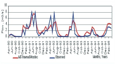
Figure 9.9 Comparison between observed and simulated monthly flow

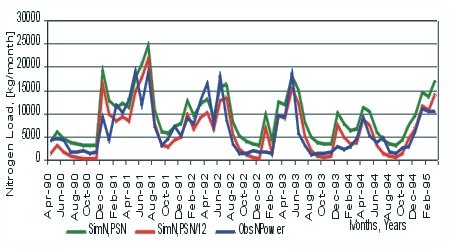
Figure 9.10 Comparison between observed and simulated monthly nitrogen load in the river

The calibration procedure is followed by the presentation of the statistical assessments and comparison between simulated and observed flow and simulated and observed nutrient loads and sediments.

9.11.2.5. Validation of the model

To validate the BISTRA model it is necessary to have the corresponding observed values. In reality there are monthly data for the validation of flow only for some points of the Yantra river. Figure 9.11 shows the situation of all the basins, used for BISTRA model validation.

Figure 9.11. Validation subbasins

The comparison between simulated and observed flow for Yantra mouth is presented in Figure 9.12.

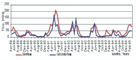
Figure 9.12 Comparison between simulated and observed flow for Yantra mouth

9.11.2.6. Output from BISTRA - input data for VODA

The output for every subbasin are: monthly precipitation, evapotranspiration, groundwater, runoff, stream flow, erosion, sediment, dissolved nitrogen and phosphorus and total nitrogen and phosphorus loads. The output values are divided in to two parts: from agricultural lands and from other lands, using the empirical dependencies and entered into proper order in input for VODA Excel file.

9.11.3 VODA - Water quality model for estimation of point source pollution

VODA is a substantial revision of the STREAMPLAN model of the International Institute of Applied Systems Analysis, developed exclusively for the basin of the Yantra River in Bulgaria. It is based on a ten years' period (1986-1995) database. REKA delivers loadings and water volume data to VODA by stream reach. VODA then computes flows and pollutant concentration and loads by reaches. The hydraulic model that underpins the VODA software assumes steady and uniform flow hydraulics in each river reach. In the water-quality model, the rate of concentration of water quality variables is assumed to be a linear function of the concentration of the water quality constituents. The socio-economic model has a pre-optimization screening procedure (for efficient operation) and an optimization step that is oriented toward in-river oxygen quantity as an indicator of river water quality.

VODA can be used to generate a scenario based on current conditions or to simulate the water quality impacts of proposed treatment facilities or discharge regulations. Alternatively, VODA can calculate financially optimal strategies to achieve water quality improvement goals or to meet specified standards for all or some of the stream reaches. Decision choices include alternative allocations of reservoir water for dilution; temporary or permanent closing of polluting entities; and capital and operational costs of pollution pre-treatment and treatment. VODA also has for input alternative weather conditions, based on the validation period or a typical wet, average, or dry year. It is also possible to include temperature and precipitation change scenarios derived from global climate change models. Typically, simulations will be framed in terms of low-flow months during relatively dry years. The numerical results of VODA's simulation and optimization are then passed back to ArcView for presentation. The results can be viewed as Excel charts and tables or as GIS-layers - ArcView shapes (Figure 9.13 and Figure 9.14).

Figure 9.13 Worst (highest) BOD - Dec/92

Figure 9.14 Best (lowest) BOD - Dec/92

In summary, it has to be mentioned that the water quality models have shown that they are the most convenient and powerful operational tools that allow to precise the water quality management policies. Nevertheless, they are always necessary to perform many various simulations of different pollutants for a given basin, to create many different scenarios for every sensitive river reach and to present the emission reduction sensitive area, which can vary with the periods of investigation and also with the meteorological weather conditions.

Bibliography

James, A. 1993. An Introduction to Water Quality Modelling, 2nd edition. John Wiley & Sons Ltd, New York.

Martin, J., and McCutcheon. 1999. Hydrodynamics and Transport for Water Quality modelling. CRC Press, New York.

Zheng, C., and B. Gordon. 1995. Applied Contaminant Transport Modelling. Van Nostrand Reinhold, New York.